def quicksort(arr):
    if len(arr) <= 1:
        return arr
    pivot = arr[len(arr) / 2]
    left = [x for x in arr if x < pivot]
    middle = [x for x in arr if x == pivot]
    right = [x for x in arr if x > pivot]
    return quicksort(left) + middle + quicksort(right)

print quicksort([3,6,8,10,1,2,1])
# Prints "[1, 1, 2, 3, 6, 8, 10]"
x = 3
print type(x) # Prints "<type 'int'>"
print x       # Prints "3"
print x + 1   # Addition; prints "4"
print x - 1   # Subtraction; prints "2"
print x * 2   # Multiplication; prints "6"
print x ** 2  # Exponentiation; prints "9"
x += 1
print x  # Prints "4"
x *= 2
print x  # Prints "8"
y = 2.5
print type(y) # Prints "<type 'float'>"
print y, y + 1, y * 2, y ** 2 # Prints "2.5 3.5 5.0 6.25"
t = True
f = False
print type(t) # Prints "<type 'bool'>"
print t and f # Logical AND; prints "False"
print t or f  # Logical OR; prints "True"
print not t   # Logical NOT; prints "False"
print t != f  # Logical XOR; prints "True"
字符串:Python对字符串的支持非常棒。
hello = 'hello'   # String literals can use single quotes
world = "world"   # or double quotes; it does not matter.
print hello       # Prints "hello"
print len(hello)  # String length; prints "5"
hw = hello + ' ' + world  # String concatenation
print hw  # prints "hello world"
hw12 = '%s %s %d' % (hello, world, 12)  # sprintf style string formatting
print hw12  # prints "hello world 12"
字符串对象有一系列有用的方法,比如:
s = "hello"
print s.capitalize()  # Capitalize a string; prints "Hello"
print s.upper()       # Convert a string to uppercase; prints "HELLO"
print s.rjust(7)      # Right-justify a string, padding with spaces; prints "  hello"
print s.center(7)     # Center a string, padding with spaces; prints " hello "
print s.replace('l', '(ell)')  # Replace all instances of one substring with another;
                               # prints "he(ell)(ell)o"
print '  world '.strip()  # Strip leading and trailing whitespace; prints "world"
xs = [3, 1, 2]   # Create a list
print xs, xs[2]  # Prints "[3, 1, 2] 2"
print xs[-1]     # Negative indices count from the end of the list; prints "2"
xs[2] = 'foo'    # Lists can contain elements of different types
print xs         # Prints "[3, 1, 'foo']"
xs.append('bar') # Add a new element to the end of the list
print xs         # Prints
x = xs.pop()     # Remove and return the last element of the list
print x, xs      # Prints "bar [3, 1, 'foo']"
nums = range(5)    # range is a built-in function that creates a list of integers
print nums         # Prints "[0, 1, 2, 3, 4]"
print nums[2:4]    # Get a slice from index 2 to 4 (exclusive); prints "[2, 3]"
print nums[2:]     # Get a slice from index 2 to the end; prints "[2, 3, 4]"
print nums[:2]     # Get a slice from the start to index 2 (exclusive); prints "[0, 1]"
print nums[:]      # Get a slice of the whole list; prints ["0, 1, 2, 3, 4]"
print nums[:-1]    # Slice indices can be negative; prints ["0, 1, 2, 3]"
nums[2:4] = [8, 9] # Assign a new sublist to a slice
print nums         # Prints "[0, 1, 8, 8, 4]"
在Numpy数组的内容中,我们会再次看到切片语法。
循环Loops:我们可以这样遍历列表中的每一个元素:
animals = ['cat', 'dog', 'monkey']
for animal in animals:
    print animal
# Prints "cat", "dog", "monkey", each on its own line.
如果想要在循环体内访问每个元素的指针,可以使用内置的enumerate函数
animals = ['cat', 'dog', 'monkey']
for idx, animal in enumerate(animals):
    print '#%d: %s' % (idx + 1, animal)
# Prints "#1: cat", "#2: dog", "#3: monkey", each on its own line
d = {'cat': 'cute', 'dog': 'furry'}  # Create a new dictionary with some data
print d['cat']       # Get an entry from a dictionary; prints "cute"
print 'cat' in d     # Check if a dictionary has a given key; prints "True"
d['fish'] = 'wet'    # Set an entry in a dictionary
print d['fish']      # Prints "wet"
# print d['monkey']  # KeyError: 'monkey' not a key of d
print d.get('monkey', 'N/A')  # Get an element with a default; prints "N/A"
print d.get('fish', 'N/A')    # Get an element with a default; prints "wet"
del d['fish']        # Remove an element from a dictionary
print d.get('fish', 'N/A') # "fish" is no longer a key; prints "N/A"
d = {'person': 2, 'cat': 4, 'spider': 8}
for animal in d:
    legs = d[animal]
    print 'A %s has %d legs' % (animal, legs)
# Prints "A person has 2 legs", "A spider has 8 legs", "A cat has 4 legs"
如果你想要访问键和对应的值,那就使用iteritems方法:
d = {'person': 2, 'cat': 4, 'spider': 8}
for animal, legs in d.iteritems():
    print 'A %s has %d legs' % (animal, legs)
# Prints "A person has 2 legs", "A spider has 8 legs", "A cat has 4 legs"
animals = {'cat', 'dog'}
print 'cat' in animals   # Check if an element is in a set; prints "True"
print 'fish' in animals  # prints "False"
animals.add('fish')      # Add an element to a set
print 'fish' in animals  # Prints "True"
print len(animals)       # Number of elements in a set; prints "3"
animals.add('cat')       # Adding an element that is already in the set does nothing
print len(animals)       # Prints "3"
animals.remove('cat')    # Remove an element from a set
print len(animals)       # Prints "2"
d = {(x, x + 1): x for x in range(10)}  # Create a dictionary with tuple keys
print d
t = (5, 6)       # Create a tuple
print type(t)    # Prints "<type 'tuple'>"
print d[t]       # Prints "5"
print d[(1, 2)]  # Prints "1"
def sign(x):
    if x > 0:
        return 'positive'
    elif x < 0:
        return 'negative'
    else:
        return 'zero'

for x in [-1, 0, 1]:
    print sign(x)
# Prints "negative", "zero", "positive"
我们常常使用可选参数来定义函数:
def hello(name, loud=False):
    if loud:
        print 'HELLO, %s' % name.upper()
    else:
        print 'Hello, %s!' % name

hello('Bob') # Prints "Hello, Bob"
hello('Fred', loud=True)  # Prints "HELLO, FRED!"
class Greeter(object):

    # Constructor
    def __init__(self, name):
        self.name = name  # Create an instance variable

    # Instance method
    def greet(self, loud=False):
        if loud:
            print 'HELLO, %s!' % self.name.upper()
        else:
            print 'Hello, %s' % self.name

g = Greeter('Fred')  # Construct an instance of the Greeter class
g.greet()            # Call an instance method; prints "Hello, Fred"
g.greet(loud=True)   # Call an instance method; prints "HELLO, FRED!"
import numpy as np

a = np.array([1, 2, 3])  # Create a rank 1 array
print type(a)            # Prints "<type 'numpy.ndarray'>"
print a.shape            # Prints "(3,)"
print a[0], a[1], a[2]   # Prints "1 2 3"
a[0] = 5                 # Change an element of the array
print a                  # Prints "[5, 2, 3]"

b = np.array([[1,2,3],[4,5,6]])   # Create a rank 2 array
print b                           # 显示一下矩阵b
print b.shape                     # Prints "(2, 3)"
print b[0, 0], b[0, 1], b[1, 0]   # Prints "1 2 4"
Numpy还提供了很多其他创建数组的方法:
import numpy as np

a = np.zeros((2,2))  # Create an array of all zeros
print a              # Prints "[[ 0.  0.]
                     #          [ 0.  0.]]"

b = np.ones((1,2))   # Create an array of all ones
print b              # Prints "[[ 1.  1.]]"

c = np.full((2,2), 7) # Create a constant array
print c               # Prints "[[ 7.  7.]
                      #          [ 7.  7.]]"

d = np.eye(2)        # Create a 2x2 identity matrix
print d              # Prints "[[ 1.  0.]
                     #          [ 0.  1.]]"

e = np.random.random((2,2)) # Create an array filled with random values
print e                     # Might print "[[ 0.91940167  0.08143941]
                            #               [ 0.68744134  0.87236687]]"
import numpy as np

# Create the following rank 2 array with shape (3, 4)
# [[ 1  2  3  4]
#  [ 5  6  7  8]
#  [ 9 10 11 12]]
a = np.array([[1,2,3,4], [5,6,7,8], [9,10,11,12]])

# Use slicing to pull out the subarray consisting of the first 2 rows
# and columns 1 and 2; b is the following array of shape (2, 2):
# [[2 3]
#  [6 7]]
b = a[:2, 1:3]

# A slice of an array is a view into the same data, so modifying it
# will modify the original array.
print a[0, 1]   # Prints "2"
b[0, 0] = 77    # b[0, 0] is the same piece of data as a[0, 1]
print a[0, 1]   # Prints "77"
import numpy as np

# Create the following rank 2 array with shape (3, 4)
# [[ 1  2  3  4]
#  [ 5  6  7  8]
#  [ 9 10 11 12]]
a = np.array([[1,2,3,4], [5,6,7,8], [9,10,11,12]])

# Two ways of accessing the data in the middle row of the array.
# Mixing integer indexing with slices yields an array of lower rank,
# while using only slices yields an array of the same rank as the
# original array:
row_r1 = a[1, :]    # Rank 1 view of the second row of a
row_r2 = a[1:2, :]  # Rank 2 view of the second row of a
print row_r1, row_r1.shape  # Prints "[5 6 7 8] (4,)"
print row_r2, row_r2.shape  # Prints "[[5 6 7 8]] (1, 4)"

# We can make the same distinction when accessing columns of an array:
col_r1 = a[:, 1]
col_r2 = a[:, 1:2]
print col_r1, col_r1.shape  # Prints "[ 2  6 10] (3,)"
print col_r2, col_r2.shape  # Prints "[[ 2]
                            #          [ 6]
                            #          [10]] (3, 1)"
import numpy as np

a = np.array([[1,2], [3, 4], [5, 6]])

# An example of integer array indexing.
# The returned array will have shape (3,) and
print a[[0, 1, 2], [0, 1, 0]]  # Prints "[1 4 5]"

# The above example of integer array indexing is equivalent to this:
print np.array([a[0, 0], a[1, 1], a[2, 0]])  # Prints "[1 4 5]"

# When using integer array indexing, you can reuse the same
# element from the source array:
print a[[0, 0], [1, 1]]  # Prints "[2 2]"

# Equivalent to the previous integer array indexing example
print np.array([a[0, 1], a[0, 1]])  # Prints "[2 2]"
整型数组访问语法还有个有用的技巧,可以用来选择或者更改矩阵中每行中的一个元素:
import numpy as np

# Create a new array from which we will select elements
a = np.array([[1,2,3], [4,5,6], [7,8,9], [10, 11, 12]])

print a  # prints "array([[ 1,  2,  3],
         #                [ 4,  5,  6],
         #                [ 7,  8,  9],
         #                [10, 11, 12]])"

# Create an array of indices
b = np.array([0, 2, 0, 1])

# Select one element from each row of a using the indices in b
print a[np.arange(4), b]  # Prints "[ 1  6  7 11]"

# Mutate one element from each row of a using the indices in b
a[np.arange(4), b] += 10

print a  # prints "array([[11,  2,  3],
         #                [ 4,  5, 16],
         #                [17,  8,  9],
         #                [10, 21, 12]])
import numpy as np

a = np.array([[1,2], [3, 4], [5, 6]])

bool_idx = (a > 2)  # Find the elements of a that are bigger than 2;
                    # this returns a numpy array of Booleans of the same
                    # shape as a, where each slot of bool_idx tells
                    # whether that element of a is > 2.

print bool_idx      # Prints "[[False False]
                    #          [ True  True]
                    #          [ True  True]]"

# We use boolean array indexing to construct a rank 1 array
# consisting of the elements of a corresponding to the True values
# of bool_idx
print a[bool_idx]  # Prints "[3 4 5 6]"

# We can do all of the above in a single concise statement:
print a[a > 2]     # Prints "[3 4 5 6]"
import numpy as np

x = np.array([1, 2])  # Let numpy choose the datatype
print x.dtype         # Prints "int64"

x = np.array([1.0, 2.0])  # Let numpy choose the datatype
print x.dtype             # Prints "float64"

x = np.array([1, 2], dtype=np.int64)  # Force a particular datatype
print x.dtype                         # Prints "int64"
import numpy as np

x = np.array([[1,2],[3,4]])

print np.sum(x)  # Compute sum of all elements; prints "10"
print np.sum(x, axis=0)  # Compute sum of each column; prints "[4 6]"
print np.sum(x, axis=1)  # Compute sum of each row; prints "[3 7]"
import numpy as np

x = np.array([[1,2],[3,4]])

print np.sum(x)  # Compute sum of all elements; prints "10"
print np.sum(x, axis=0)  # Compute sum of each column; prints "[4 6]"
print np.sum(x, axis=1)  # Compute sum of each row; prints "[3 7]"
import numpy as np

# We will add the vector v to each row of the matrix x,
# storing the result in the matrix y
x = np.array([[1,2,3], [4,5,6], [7,8,9], [10, 11, 12]])
v = np.array([1, 0, 1])
y = np.empty_like(x)   # Create an empty matrix with the same shape as x

# Add the vector v to each row of the matrix x with an explicit loop
for i in range(4):
    y[i, :] = x[i, :] + v

# Now y is the following
# [[ 2  2  4]
#  [ 5  5  7]
#  [ 8  8 10]
#  [11 11 13]]
print y
这样是行得通的,但是当x矩阵非常大,利用循环来计算就会变得很慢很慢。我们可以换一种思路:
import numpy as np

# We will add the vector v to each row of the matrix x,
# storing the result in the matrix y
x = np.array([[1,2,3], [4,5,6], [7,8,9], [10, 11, 12]])
v = np.array([1, 0, 1])
vv = np.tile(v, (4, 1))  # Stack 4 copies of v on top of each other
print vv                 # Prints "[[1 0 1]
                         #          [1 0 1]
                         #          [1 0 1]
                         #          [1 0 1]]"
y = x + vv  # Add x and vv elementwise
print y  # Prints "[[ 2  2  4
         #          [ 5  5  7]
         #          [ 8  8 10]
         #          [11 11 13]]"
Numpy广播机制可以让我们不用创建vv,就能直接运算,看看下面例子:
import numpy as np

# We will add the vector v to each row of the matrix x,
# storing the result in the matrix y
x = np.array([[1,2,3], [4,5,6], [7,8,9], [10, 11, 12]])
v = np.array([1, 0, 1])
y = x + v  # Add v to each row of x using broadcasting
print y  # Prints "[[ 2  2  4]
         #          [ 5  5  7]
         #          [ 8  8 10]
         #          [11 11 13]]"
import numpy as np

# Compute outer product of vectors
v = np.array([1,2,3])  # v has shape (3,)
w = np.array([4,5])    # w has shape (2,)
# To compute an outer product, we first reshape v to be a column
# vector of shape (3, 1); we can then broadcast it against w to yield
# an output of shape (3, 2), which is the outer product of v and w:
# [[ 4  5]
#  [ 8 10]
#  [12 15]]
print np.reshape(v, (3, 1)) * w

# Add a vector to each row of a matrix
x = np.array([[1,2,3], [4,5,6]])
# x has shape (2, 3) and v has shape (3,) so they broadcast to (2, 3),
# giving the following matrix:
# [[2 4 6]
#  [5 7 9]]
print x + v

# Add a vector to each column of a matrix
# x has shape (2, 3) and w has shape (2,).
# If we transpose x then it has shape (3, 2) and can be broadcast
# against w to yield a result of shape (3, 2); transposing this result
# yields the final result of shape (2, 3) which is the matrix x with
# the vector w added to each column. Gives the following matrix:
# [[ 5  6  7]
#  [ 9 10 11]]
print (x.T + w).T

# Another solution is to reshape w to be a row vector of shape (2, 1);
# we can then broadcast it directly against x to produce the same
# output.
print x + np.reshape(w, (2, 1))

# Multiply a matrix by a constant:
# x has shape (2, 3). Numpy treats scalars as arrays of shape ();
# these can be broadcast together to shape (2, 3), producing the
# following array:
# [[ 2  4  6]
#  [ 8 10 12]]
print x * 2
from scipy.misc import imread, imsave, imresize

# Read an JPEG image into a numpy array
img = imread('assets/cat.jpg')
print img.dtype, img.shape  # Prints "uint8 (400, 248, 3)"

# We can tint the image by scaling each of the color channels
# by a different scalar constant. The image has shape (400, 248, 3);
# we multiply it by the array [1, 0.95, 0.9] of shape (3,);
# numpy broadcasting means that this leaves the red channel unchanged,
# and multiplies the green and blue channels by 0.95 and 0.9
# respectively.
img_tinted = img * [1, 0.95, 0.9]

# Resize the tinted image to be 300 by 300 pixels.
img_tinted = imresize(img_tinted, (300, 300))

# Write the tinted image back to disk
imsave('assets/cat_tinted.jpg', img_tinted)
译者注:如果运行这段代码出现类似ImportError: cannot import name imread的报错,那么请利用pip进行Pillow的下载,可以解决问题。命令:pip install Pillow。
import numpy as np
from scipy.spatial.distance import pdist, squareform

# Create the following array where each row is a point in 2D space:
# [[0 1]
#  [1 0]
#  [2 0]]
x = np.array([[0, 1], [1, 0], [2, 0]])
print x

# Compute the Euclidean distance between all rows of x.
# d[i, j] is the Euclidean distance between x[i, :] and x[j, :],
# and d is the following array:
# [[ 0.          1.41421356  2.23606798]
#  [ 1.41421356  0.          1.        ]
#  [ 2.23606798  1.          0.        ]]
d = squareform(pdist(x, 'euclidean'))
print d
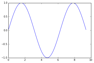
import numpy as np
import matplotlib.pyplot as plt

# Compute the x and y coordinates for points on a sine curve
x = np.arange(0, 3 * np.pi, 0.1)
y = np.sin(x)

# Plot the points using matplotlib
plt.plot(x, y)
plt.show()  # You must call plt.show() to make graphics appear.
运行上面代码会产生下面的作图:
—————————————————————————————————————————
—————————————————————————————————————————
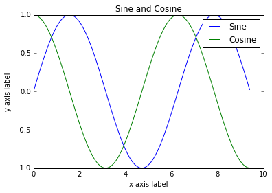
只需要少量工作,就可以一次画不同的线,加上标签,坐标轴标志等。
import numpy as np
import matplotlib.pyplot as plt

# Compute the x and y coordinates for points on sine and cosine curves
x = np.arange(0, 3 * np.pi, 0.1)
y_sin = np.sin(x)
y_cos = np.cos(x)

# Plot the points using matplotlib
plt.plot(x, y_sin)
plt.plot(x, y_cos)
plt.xlabel('x axis label')
plt.ylabel('y axis label')
plt.title('Sine and Cosine')
plt.legend(['Sine', 'Cosine'])
plt.show()
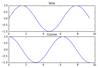
import numpy as np
import matplotlib.pyplot as plt

# Compute the x and y coordinates for points on sine and cosine curves
x = np.arange(0, 3 * np.pi, 0.1)
y_sin = np.sin(x)
y_cos = np.cos(x)

# Set up a subplot grid that has height 2 and width 1,
# and set the first such subplot as active.
plt.subplot(2, 1, 1)

# Make the first plot
plt.plot(x, y_sin)
plt.title('Sine')

# Set the second subplot as active, and make the second plot.
plt.subplot(2, 1, 2)
plt.plot(x, y_cos)
plt.title('Cosine')

# Show the figure.
plt.show()
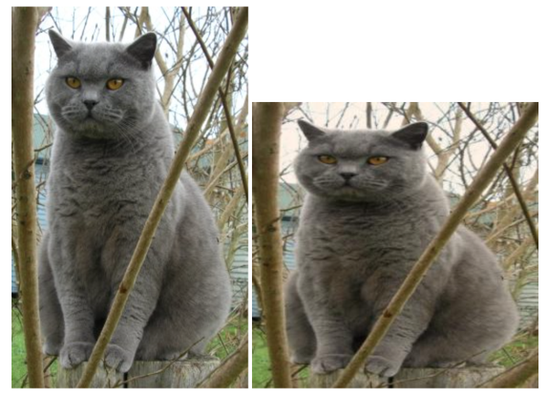
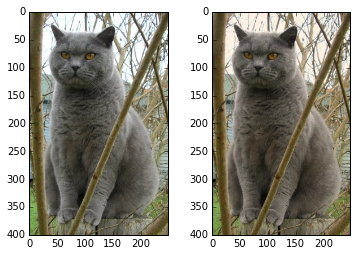
import numpy as np
from scipy.misc import imread, imresize
import matplotlib.pyplot as plt

img = imread('assets/cat.jpg')
img_tinted = img * [1, 0.95, 0.9]

# Show the original image
plt.subplot(1, 2, 1)
plt.imshow(img)

# Show the tinted image
plt.subplot(1, 2, 2)

# A slight gotcha with imshow is that it might give strange results
# if presented with data that is not uint8. To work around this, we
# explicitly cast the image to uint8 before displaying it.
plt.imshow(np.uint8(img_tinted))
plt.show()
conda update anaconda 后提示
1ValueError: unsupported format character ')' (0x29) at index 49 查到了这个:anaconda update issue
I have narrowed this down to the following packages:
package build psutil-1.2.1 py27_0 hard-link pycparser-2.10 py27_0 hard-link pykit-0.1.0 np18py27_2 hard-link pyparsing-2.0.1 py27_0 hard-link by calling "conda install anaconda" and then successfully installing everything else one at a time. These four packages consistently exhibit the described behaviour. (note: pykit depends on pycparser so may itself be ok - can't tell) 我先把psutil卸载掉,重新update了一下,成功。
参考资料:install qq/tim on linux with wine
wine运行qq不能输入账号
This tutorial introduces how to install QQ/TIM in Linux with Wine, which had been tested on ArchLinux with Wine 2.4.