背景#
虽然不太care 训练的过程,但是由于容易看懂的layer都看得差不多了 所以打算看一下这些loss function.
Euclidean Loss (L2 loss)#
一般用于 “real-valued regression tasks”。比如之前项目里用的人脸年龄模型,就是用了这个 Loss。
这个 loss 没什么额外的参数,实现也很简单。
 1
 2template <typename Dtype>
 3void EuclideanLossLayer<Dtype>::Reshape(
 4  const vector<Blob<Dtype>*>& bottom, const vector<Blob<Dtype>*>& top) {
 5  LossLayer<Dtype>::Reshape(bottom, top);
 6  CHECK_EQ(bottom[0]->count(1), bottom[1]->count(1))
 7      << "Inputs must have the same dimension.";
 8  diff_.ReshapeLike(*bottom[0]);
 9}
10
11template <typename Dtype>
12void EuclideanLossLayer<Dtype>::Forward_cpu(const vector<Blob<Dtype>*>& bottom,
13    const vector<Blob<Dtype>*>& top) {
14  int count = bottom[0]->count();
15  caffe_sub(
16      count,
17      bottom[0]->cpu_data(),
18      bottom[1]->cpu_data(),
19      diff_.mutable_cpu_data());
20  Dtype dot = caffe_cpu_dot(count, diff_.cpu_data(), diff_.cpu_data());
21  Dtype loss = dot / bottom[0]->num() / Dtype(2);
22  top[0]->mutable_cpu_data()[0] = loss;
23}
注意 Reshape 中要求两个 bottom blob(第一个为预测结果,第二个为 gt)的 batch 维度可以不同,计算时按照预测结果的个数为准。
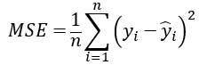
以及,Mean Square Error(MSE)和 L2 loss 的差别只是一个系数 1/2,可以放在一起说明。
MultinomialLogisticLoss#
用于单标签多分类任务。输入的预测 blob 是一个(通常经过 softmax 后得到的)概率分布。
注意 “The SoftmaxWithLossLayer should be preferred over separate SoftmaxLayer + MultinomialLogisticLossLayer as its gradient computation is more numerically stable.”
这个后面会提到。
同样,这个 loss 也没什么额外参数,forward 也很简单:
 1
 2template <typename Dtype>
 3void MultinomialLogisticLossLayer<Dtype>::Forward_cpu(
 4    const vector<Blob<Dtype>*>& bottom, const vector<Blob<Dtype>*>& top) {
 5  const Dtype* bottom_data = bottom[0]->cpu_data();
 6  //  predictions, NxCxHxW
 7  const Dtype* bottom_label = bottom[1]->cpu_data();
 8  // labels, Nx1x1x1
 9  int num = bottom[0]->num();
10  int dim = bottom[0]->count() / bottom[0]->num();
11  // dim 表示类别总数
12  Dtype loss = 0;
13  //  bottom_data[i * dim + label]表示的是第i张图的gt对应的位置的预测分数
14  for (int i = 0; i < num; ++i) {
15    int label = static_cast<int>(bottom_label[i]);
16    Dtype prob = std::max(
17        bottom_data[i * dim + label], Dtype(kLOG_THRESHOLD));
18    loss -= log(prob);
19  }
20  top[0]->mutable_cpu_data()[0] = loss / num;
21}
需要注意的已经写在注释中了。 kLOG_THRESHOLD 是一个很小的值 1E-20,防止 log0 炸掉。
hinge-loss#
\[ \ell (y)=\max(0,1-t\cdot y) \]中文似乎叫 “合页损失函数”,因为很像一本书打开的样子(?
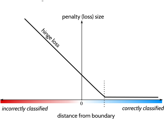
主要用在 svm 中,所以其实没在工作中实际接触过这个。
这个 loss 的特点是更加严格,严格的意思是说:分类的结果不仅需要正确,而且需要置信度足够高,损失才会是 0。
forward 代码稍微不是那么直接:
 1
 2  const Dtype* bottom_data = bottom[0]->cpu_data();
 3  Dtype* bottom_diff = bottom[0]->mutable_cpu_diff();
 4  const Dtype* label = bottom[1]->cpu_data();
 5  int num = bottom[0]->num();
 6  int count = bottom[0]->count();
 7  int dim = count / num;
 8  // dim是类别数
 9
10  caffe_copy(count, bottom_data, bottom_diff);
11  // 把预测值bottom_data拷贝到bottom_diff
12  for (int i = 0; i < num; ++i) {
13    bottom_diff[i * dim + static_cast<int>(label[i])] *= -1;
14  }
15  // 把gt的那一类的预测分数取了相反数(这里相当于算了condition函数,只不过差个负号)
16
17  for (int i = 0; i < num; ++i) {
18    for (int j = 0; j < dim; ++j) {
19      bottom_diff[i * dim + j] = std::max(
20        Dtype(0), 1 + bottom_diff[i * dim + j]);
21    }
先算了一个 bottom_diff,这里其实相当于算了 condition function 的结果,只不过差了一个负号。后面可以看到,代码里计算的就是:
1
2bottom_diff[i * dim + j] = std::max(
3        Dtype(0), 1 + bottom_diff[i * dim + j]);
还值得一提的是,caffe 的 hinge loss 同时支持 L1 norm 和 L2 norm(在 L2-SVM 中使用)。
 1message HingeLossParameter {
 2  enum Norm {
 3    L1 = 1;
 4    L2 = 2;
 5  }
 6  // Specify the Norm to use L1 or L2
 7  optional Norm norm = 1 [default = L1];
 8}
 9
10
11
12  Dtype* loss = top[0]->mutable_cpu_data();
13  switch (this->layer_param_.hinge_loss_param().norm()) {
14  case HingeLossParameter_Norm_L1:
15    loss[0] = caffe_cpu_asum(count, bottom_diff) / num;
16    break;
17  case HingeLossParameter_Norm_L2:
18    loss[0] = caffe_cpu_dot(count, bottom_diff, bottom_diff) / num;
19    break;
20  default:
21    LOG(FATAL) << "Unknown Norm";
22  }
23}